Using MATLAB to Investigate the Relationship Between Lifestyle Factors and Blood Pressure: Multiple Regression and ANOVA

Julia Huang

Introduction

Hypertension is one of the leading risk factors for cardiovascular disease, affecting millions of adults worldwide. Elevated blood pressure increases the risk of heart disease, stroke, and kidney disease, which is why I consider it such a critical public health concern. Because blood pressure is influenced by a mix of biological and behavioral factors, I’ve noticed researchers focusing more on lifestyle interventions to improve control.

Recent evidence suggests that it’s not just what we do, but when we do it that matters for cardiovascular health. I was particularly interested in a 2024 systematic review by Keiser et al., which looked at how the timing of eating, exercise, and sleep impacts blood pressure. They found that earlier eating schedules, proper sleep timing, and specific exercise windows often led to better outcomes. Inspired by these findings, I decided to use MATLAB to investigate the relationship between lifestyle variables and blood pressure myself. I used multiple linear regression to see how several variables predict blood pressure together, and one-way ANOVA to compare blood pressure across different age groups.

Background

I’ve always found the concept of “chronobehavior” fascinating—the idea that when we eat, move, or sleep might be just as important as the behaviors themselves. Keiser et al. (2024) provided a strong motivation for my analysis, even though they noted that current evidence is still limited by differences in study designs.

In this project, I’m using MATLAB to walk through a full statistical workflow, from importing raw health data to interpreting the final results. My goal is to show how these statistical methods can provide practical insights into real-world health data.

MATLAB Tutorial: Preparing and Analyzing NHANES Data

This section demonstrates how MATLAB was used to import, clean, merge, and analyze data from the 2017–2018 National Health and Nutrition Examination Survey (NHANES). The analysis focuses on systolic blood pressure and its relationship with age, BMI, sleep duration, and sex. Multiple linear regression was used to examine the combined effects of these variables, while one-way ANOVA was used to compare systolic blood pressure among different age groups.

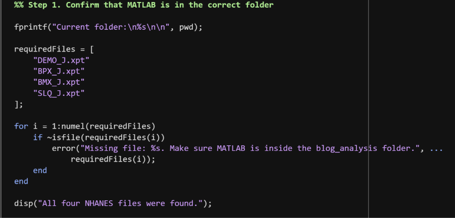
Step 1. Confirm the Current Folder

Before importing the data, MATLAB first checks the current working folder. All four NHANES data files and the MATLAB script must be stored in the same project folder.

fprintf(“Current folder:\n%s\n\n”, pwd);

The pwd function displays the current folder location. This helps prevent file path errors when MATLAB attempts to open the datasets.

The program then creates a list of the four required files:

requiredFiles = [
   “DEMO_J.xpt”
   “BPX_J.xpt”
   “BMX_J.xpt”
   “SLQ_J.xpt”
];

A for loop checks whether every file exists in the folder.

for i = 1:numel(requiredFiles)
   if ~isfile(requiredFiles(i))
       error(“Missing file: %s. Make sure MATLAB is inside the blog_analysis folder.”, …
           requiredFiles(i));
   end
end

If a file is missing, MATLAB stops the program and displays an error message. This verification step prevents the analysis from continuing with incomplete data.

Step 2. Import the SAS XPORT Files

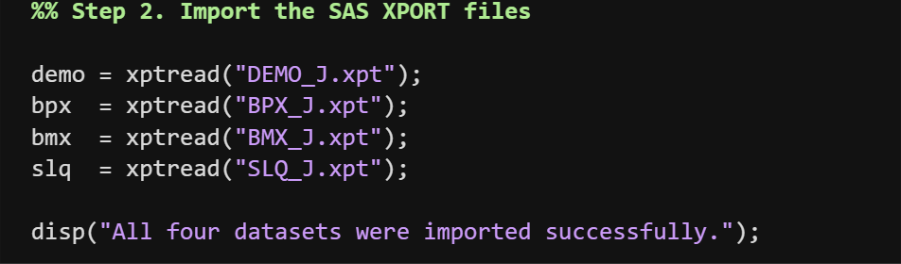
NHANES datasets are distributed as SAS XPORT files with the .xpt extension. The four files were imported into MATLAB using the xptread function.

demo = xptread(“DEMO_J.xpt”);
bpx = xptread(“BPX_J.xpt”);
bmx = xptread(“BMX_J.xpt”);
slq = xptread(“SLQ_J.xpt”);

Each imported file becomes a MATLAB table:

MATLAB table	NHANES dataset	Information used
demo	Demographics	Age and sex
bpx	Blood Pressure	Systolic blood pressure measurements
bmx	Body Measures	Body mass index
slq	Sleep Questionnaire	Sleep duration

MATLAB tables preserve the original NHANES variable names, making it easier to select and merge the required information.

Step 3. Display the Size of Each Dataset

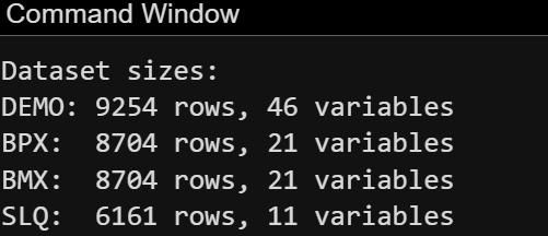
After importing the files, the number of rows and variables in each dataset was displayed.

fprintf(“DEMO: %d rows, %d variables\n”, height(demo), width(demo));
fprintf(“BPX: %d rows, %d variables\n”, height(bpx), width(bpx));
fprintf(“BMX: %d rows, %d variables\n”, height(bmx), width(bmx));
fprintf(“SLQ: %d rows, %d variables\n”, height(slq), width(slq));

The height function returns the number of observations, while width returns the number of variables.

This step confirms that the datasets were imported correctly and gives an initial understanding of their dimensions. The datasets may contain different numbers of rows because not every NHANES participant completed every examination or questionnaire.

Step 4. Check the Required Variable Names

Before selecting variables, the program verifies that the required columns exist.

requiredDemo = [“SEQN”,”RIDAGEYR”,”RIAGENDR”];
requiredBMX = [“SEQN”,”BMXBMI”];
requiredBPX = [“SEQN”,”BPXSY1″,”BPXSY2″,”BPXSY3″,”BPXSY4″];

The variables used in this project include:

Variable	Description
SEQN	Participant identification number
RIDAGEYR	Age in years
RIAGENDR	Sex
BMXBMI	Body mass index
BPXSY1–BPXSY4	Repeated systolic blood pressure measurements

The custom checkVariables function compares the required variable names with the variables available in each table.

checkVariables(demo, requiredDemo, “DEMO_J”);
checkVariables(bmx, requiredBMX, “BMX_J”);

For blood pressure, the program identifies which systolic blood pressure measurements are available.

allSBPVariables = [“BPXSY1″,”BPXSY2″,”BPXSY3″,”BPXSY4”];

availableSBP = allSBPVariables( …
ismember(allSBPVariables, string(bpx.Properties.VariableNames)));

This approach makes the code more flexible because some participants may not have all four blood pressure readings.

Step 5. Identify the Sleep-Duration Variable

The exact name of the sleep-duration variable may differ between NHANES survey cycles. The program therefore checks several possible variable names.

sleepCandidates = [
   “SLD012”
   “SLD013”
   “SLD010H”
   “SLD012H”
];

MATLAB compares these candidate names with the variables found in the sleep questionnaire dataset.

availableSleep = sleepCandidates( …
ismember(sleepCandidates, string(slq.Properties.VariableNames)));

The first available sleep-duration variable is selected:

sleepVariable = availableSleep(1);

This method avoids manually changing the code when a different NHANES cycle uses a slightly different variable name.

Step 6. Keep Only the Variables Needed for Analysis

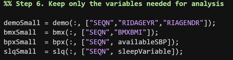
The original NHANES datasets contain many variables that are not necessary for this project. To simplify the analysis, smaller tables were created containing only the required variables.

demoSmall = demo(:, [“SEQN”,”RIDAGEYR”,”RIAGENDR”]);
bmxSmall = bmx(:, [“SEQN”,”BMXBMI”]);
bpxSmall = bpx(:, [“SEQN”, availableSBP]);
slqSmall = slq(:, [“SEQN”, sleepVariable]);

Reducing the datasets has several advantages. It makes the tables easier to inspect, reduces memory use, and decreases the possibility of accidentally including unrelated variables in the statistical model.

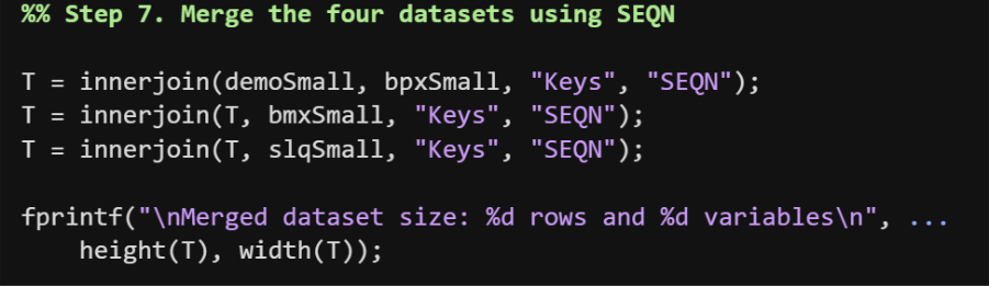
Step 7. Merge the Four Datasets Using SEQN

NHANES stores different categories of participant information in separate files. The participant identification number, SEQN, was used to combine the four datasets.

T = innerjoin(demoSmall, bpxSmall, “Keys”, “SEQN”);
T = innerjoin(T, bmxSmall, “Keys”, “SEQN”);
T = innerjoin(T, slqSmall, “Keys”, “SEQN”);

The innerjoin function keeps participants who appear in both tables being merged. After all four joins are completed, each row contains demographic, blood pressure, BMI, and sleep information for one participant.

Participants who did not have records in all four datasets were excluded during the merge. The final dimensions of the merged table were displayed using height and width.

Step 8. Calculate Average Systolic Blood Pressure

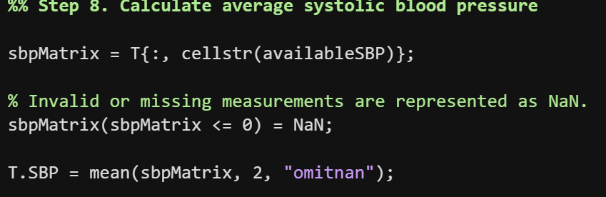
NHANES records several systolic blood pressure measurements for many participants. Using only one measurement could be affected by temporary variation or measurement error. Therefore, the available systolic blood pressure readings were averaged.

sbpMatrix = T{:, cellstr(availableSBP)};

This command extracts the blood pressure columns from the table and converts them into a numeric matrix.

Invalid measurements were converted to missing values:

sbpMatrix(sbpMatrix <= 0) = NaN;

The average systolic blood pressure was then calculated for each participant.

T.SBP = mean(sbpMatrix, 2, “omitnan”);

The value 2 tells MATLAB to calculate the mean across columns for each row. The “omitnan” option allows MATLAB to calculate an average even when one or more readings are missing.

The new variable SBP represents average systolic blood pressure in millimeters of mercury.

Step 9. Rename the Variables

The original NHANES variable names are useful for documentation, but descriptive names make the analysis easier to understand.

T.Properties.VariableNames( …
   strcmp(T.Properties.VariableNames,”RIDAGEYR”)) = {‘Age’};

T.Properties.VariableNames( …
   strcmp(T.Properties.VariableNames,”RIAGENDR”)) = {‘Sex’};

T.Properties.VariableNames( …
   strcmp(T.Properties.VariableNames,”BMXBMI”)) = {‘BMI’};

T.Properties.VariableNames( …
   strcmp(T.Properties.VariableNames,char(sleepVariable))) = {‘SleepHours’};

The variables were renamed as follows:

Original name	New name
RIDAGEYR	Age
RIAGENDR	Sex
BMXBMI	BMI
Sleep variable	SleepHours

These names are easier to interpret in regression equations, figures, and output tables.

Step 10. Convert Sex Codes into Labels

In NHANES, sex is stored as numeric codes. The code 1 represents male participants and 2 represents female participants.

The numeric values were converted into categorical labels:

T.Sex = categorical(T.Sex, [1 2], [“Male”,”Female”]);

Categorical variables are useful in regression analysis because MATLAB automatically creates the necessary indicator variable when fitting the model.

This also makes the final dataset easier to read because it displays Male and Female instead of numeric codes.

Step 11. Keep Adults Only

This project focuses on blood pressure among adults. Participants younger than 18 years were excluded.

T = T(T.Age >= 18, :);

The logical condition T.Age >= 18 identifies adult participants. The colon keeps all variables for the selected rows.

Restricting the sample to adults also makes the analysis more consistent with the study by Keiser et al. (2024), which examined blood pressure and lifestyle behaviors among adult populations.

Step 12. Clean Invalid and Missing Values

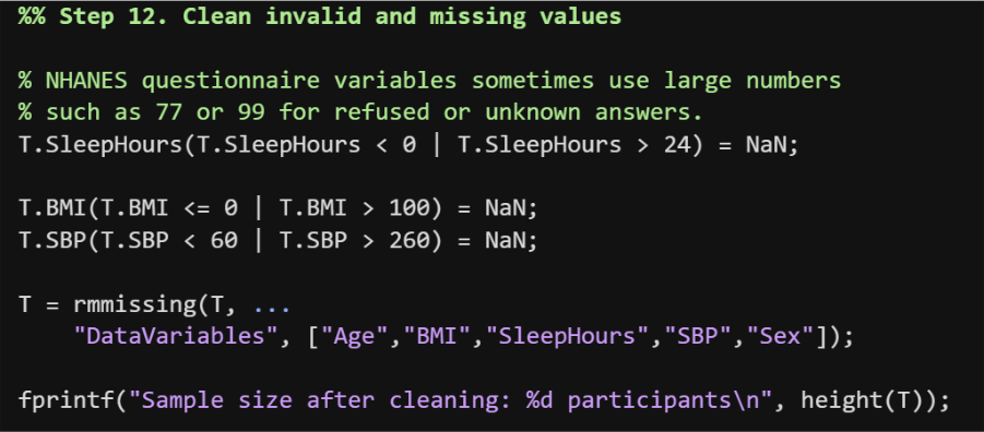
Health datasets frequently contain missing, refused, unknown, or biologically implausible values. These values must be addressed before performing statistical analysis.

Sleep duration values below zero or above 24 hours were treated as missing:

T.SleepHours(T.SleepHours < 0 | T.SleepHours > 24) = NaN;

BMI values outside the selected plausible range were also replaced with missing values:

T.BMI(T.BMI <= 0 | T.BMI > 100) = NaN;

Similarly, implausible systolic blood pressure values were removed:

T.SBP(T.SBP < 60 | T.SBP > 260) = NaN;

Participants missing any variable required for the analysis were then removed.

T = rmmissing(T, …
“DataVariables”, [“Age”,”BMI”,”SleepHours”,”SBP”,”Sex”]);

This creates a complete-case dataset in which every remaining participant has valid values for all regression variables.

The program displays the number of participants remaining after cleaning:

fprintf(“Sample size after cleaning: %d participants\n”, height(T));

Step 13. Create Age Groups for One-Way ANOVA

To compare systolic blood pressure among different age groups, age was converted from a continuous variable into three categories.

ageEdges = [18 40 60 Inf];

ageLabels = …
[“Young Adults”,”Middle-Aged Adults”,”Older Adults”];

The groups were defined as:

Age group	Range
Young Adults	18–39 years
Middle-Aged Adults	40–59 years
Older Adults	60 years or older

The discretize function assigned each participant to the appropriate category.

T.AgeGroup = discretize( …
   T.Age, …
   ageEdges, …
   “categorical”, …
   ageLabels);

The resulting categorical variable, AgeGroup, was later used as the grouping variable in the one-way ANOVA.

Step 14. Create the Final Analysis Table

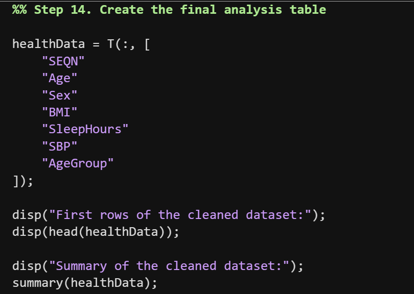
After merging and cleaning the data, a final table was created containing only the variables needed for the statistical analysis.

healthData = T(:, [
   “SEQN”
   “Age”
   “Sex”
   “BMI”
   “SleepHours”
   “SBP”
   “AgeGroup”
]);

The final table contains:

Variable	Role
SEQN	Participant identification number
Age	Continuous regression predictor
Sex	Categorical regression predictor
BMI	Continuous regression predictor
SleepHours	Lifestyle-related regression predictor
SBP	Dependent variable
AgeGroup	ANOVA grouping variable

The first rows of the final table were displayed using:

disp(head(healthData));

The summary function was also used to examine each variable.

summary(healthData);

Step 15. Export the Cleaned Dataset

The cleaned dataset was saved as a CSV file.

writetable(healthData, “health_data.csv”);

Saving the prepared dataset has several benefits. The cleaned data can be reopened without repeating the import and merging process, shared with others, and used for future analyses.

The exported file also improves reproducibility because it preserves the exact data used in the regression and ANOVA.

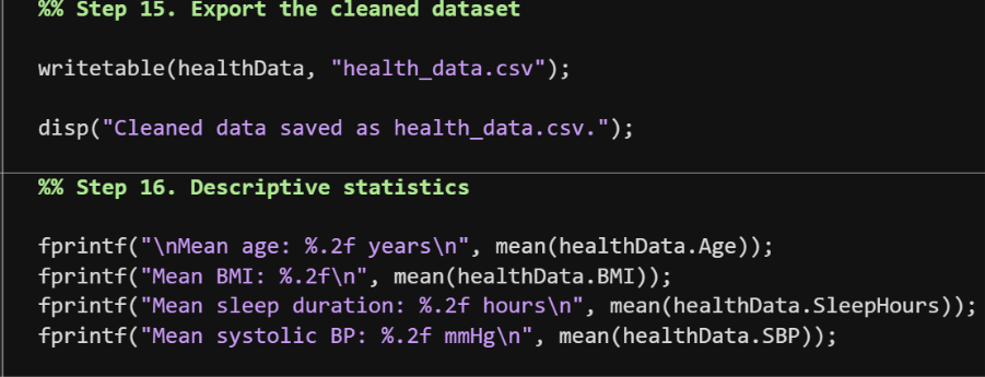
Step 16. Calculate Descriptive Statistics

Before fitting statistical models, descriptive statistics were calculated to summarize the characteristics of the sample.

fprintf(“\nMean age: %.2f years\n”, mean(healthData.Age));
fprintf(“Mean BMI: %.2f\n”, mean(healthData.BMI));
fprintf(“Mean sleep duration: %.2f hours\n”, mean(healthData.SleepHours));
fprintf(“Mean systolic BP: %.2f mmHg\n”, mean(healthData.SBP));

The program calculates:

Mean age

Mean BMI

Mean sleep duration

Mean systolic blood pressure

The format %.2f displays each result with two decimal places.

Step 17. Perform Multiple Linear Regression

Multiple linear regression was used to examine how age, BMI, sleep duration, and sex were jointly associated with systolic blood pressure.

mdl = fitlm(healthData, …
“SBP ~ Age + BMI + SleepHours + Sex”);

The dependent variable was average systolic blood pressure. The predictors were:

Sleep duration

The regression model can be represented conceptually as:

The fitlm function estimates the regression coefficients and provides several important statistics:

Estimated coefficient

Standard error

t-statistic

p-value

R-squared

Adjusted R-squared

Overall F-test

The model output was displayed using:

disp(mdl);

An ANOVA table for the regression model was also generated:

disp(anova(mdl, “summary”));

A predictor with a p-value below 0.05 was interpreted as statistically significantly associated with systolic blood pressure after controlling for the other variables in the model.

However, because this analysis uses observational survey data, statistically significant associations should not automatically be interpreted as causal effects.

Step 18. Plot Regression Diagnostics

Regression diagnostics were used to evaluate whether the assumptions of the multiple linear regression model were reasonable.

The first plot displays residuals against fitted values:

figure;
plotResiduals(mdl, “fitted”);
title(“Residuals versus Fitted Values”);

Residuals represent the differences between observed and model-predicted systolic blood pressure values.

A reasonable model should show residuals distributed randomly around zero. A curved pattern may suggest nonlinearity, while a widening pattern may indicate unequal residual variance.

The second plot examines the normality of the residuals:

figure;
plotResiduals(mdl, “probability”);
title(“Normal Probability Plot of Residuals”);

If the residuals are approximately normally distributed, the plotted points should follow the reference line reasonably closely. Large deviations may indicate outliers or non-normal residuals.

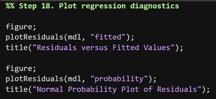
Figure 1. Residuals versus Fitted Values

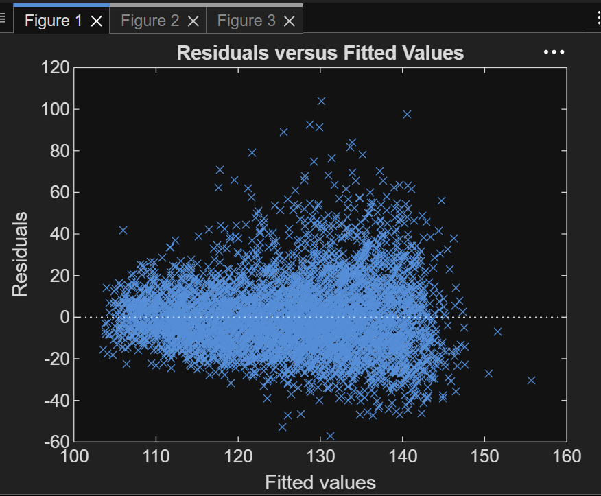
The residuals are generally centered around the horizontal zero line, indicating that the model does not exhibit a strong systematic bias. However, the spread of the residuals increases as the fitted values become larger, suggesting some degree of heteroscedasticity. In addition, several observations have relatively large residuals, indicating the presence of potential outliers.

Although these patterns suggest that the regression assumptions are not perfectly satisfied, the large sample size provides reasonable robustness for the overall regression analysis.

Figure 2. Normal Probability Plot of Residuals

The normal probability plot was used to assess whether the residuals followed an approximately normal distribution. Most observations lie close to the reference line in the middle portion of the plot, while noticeable deviations appear in the tails. This indicates that the residuals are approximately normal but contain several extreme observations. Given the large number of participants included in this study, these departures from normality are unlikely to substantially affect the validity of the regression results.

Step 19. Perform One-Way ANOVA

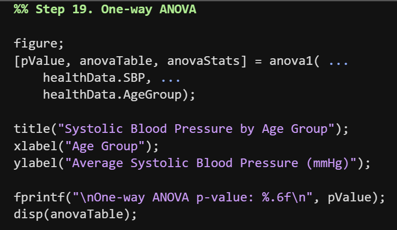
A one-way analysis of variance was used to test whether mean systolic blood pressure differed among the three age groups.

[pValue, anovaTable, anovaStats] = anova1( …
healthData.SBP, …
healthData.AgeGroup);

The hypotheses were:

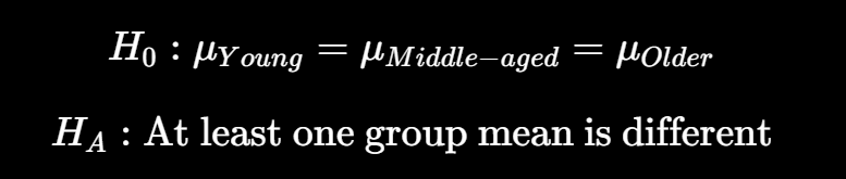
The ANOVA compares variation between age groups with variation within age groups.

The output includes:

Sum of squares

Degrees of freedom

Mean square

F-statistic

p-value

The anova1 function also produces a boxplot showing the distribution of systolic blood pressure in each age group.

The interpretation is:

If p < 0.05, reject the null hypothesis.

If p ≥ 0.05, there is insufficient evidence that the age-group means differ.

Figure 5. Systolic Blood Pressure by Age Group

The boxplot provides a visual comparison of systolic blood pressure across the three age groups. The median systolic blood pressure increases steadily from young adults to middle-aged adults and reaches the highest level among older adults. Older adults also show greater variability and more extreme values, indicating a wider distribution of blood pressure measurements within this group.

Step 20. Conduct Post-Hoc Comparisons

A statistically significant ANOVA indicates that at least one group differs, but it does not identify which specific groups are different.

Therefore, post-hoc pairwise comparisons were performed only when the ANOVA p-value was below 0.05.

if pValue < 0.05
   figure;
   comparisonResults = multcompare(anovaStats);
   title(“Post-Hoc Comparisons Between Age Groups”);

   disp(“Post-hoc comparison results:”);
   disp(comparisonResults);
end

The multcompare function compares:

Young adults versus middle-aged adults

Young adults versus older adults

Middle-aged adults versus older adults

For each comparison, MATLAB provides the estimated difference and confidence interval.

When the confidence interval does not include zero, the two group means are considered statistically significantly different.

If the ANOVA result is not significant, the program does not perform post-hoc comparisons because there is no overall evidence of a group difference.

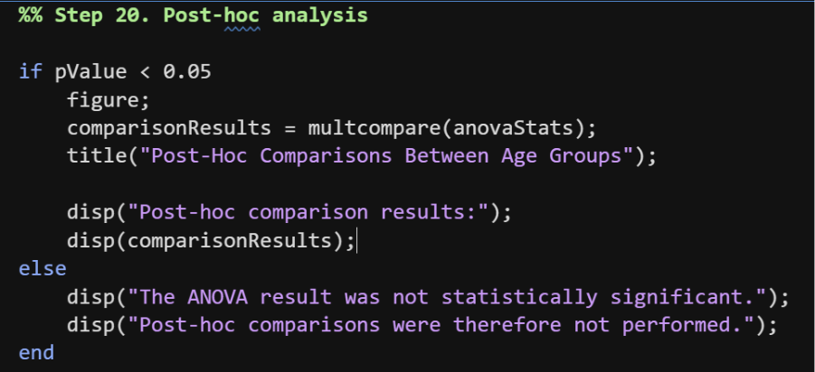
Figure 6. Post-Hoc Comparisons Between Age Groups

The post-hoc analysis indicates that the mean systolic blood pressure of both the middle-aged and older adult groups differs significantly from that of the young adult group. The older adult group exhibits the highest average systolic blood pressure, while the young adult group has the lowest average. These findings are consistent with the overall ANOVA result and suggest that systolic blood pressure increases with age.

Results

After cleaning everything up, my final dataset included 5,142 adult participants. I calculated the descriptive statistics—like average age, BMI, and sleep duration—directly from the NHANES data before moving on to the actual models.

Multiple Linear Regression

I ran a multiple linear regression to see how age, BMI, sleep duration, and sex work together to predict systolic blood pressure. Overall, the model was statistically significant and explained about 26% of the variability in blood pressure. This tells me that demographic and lifestyle factors definitely play a huge role.

Age was the strongest predictor—older participants clearly tended to have higher blood pressure. BMI also had a positive link, and sex remained a significant factor even after I adjusted for everything else. Interestingly, sleep duration on its own didn’t stand out as a significant predictor once I controlled for the other variables.

Regression Diagnostics

I checked my assumptions using diagnostic plots. The residual-versus-fitted plot showed that the residuals were mostly centered around zero, though the spread got a bit wider at higher values, suggesting some mild heteroscedasticity and a few outliers. The normal probability plot showed that the residuals were mostly normal, especially in the middle, despite some extreme values in the tails. Given the large sample size, I’m confident these minor deviations won’t throw off the overall results.

One-Way ANOVA

Next, I used a one-way ANOVA to compare blood pressure across my three age groups. The results showed a huge difference (F(2,5139)=674.1,p<0.001), so I rejected the idea that all age groups have the same mean blood pressure. The boxplots made this trend very obvious: median blood pressure climbed steadily from young adults to middle-aged adults, hitting its peak with the older group.

Post-Hoc Comparisons

Since the ANOVA was significant, I followed up with Tukey’s post-hoc test. This confirmed that both the middle-aged and older groups had significantly higher average blood pressure than the younger group. It’s a very clear signal that systolic blood pressure increases substantially as we age.

Discussion

My findings line up with what we already know: age is one of the biggest predictors of blood pressure because vessels lose elasticity over time. The positive link with BMI also matches previous studies showing how weight increases the workload on the heart.

As for sleep, the fact that duration wasn’t significant doesn’t mean sleep doesn’t matter. It just suggests that “hours slept” doesn’t tell the whole story. As Keiser et al. (2024) noted, the timing of sleep, eating, and exercise might be more important than just the duration.

Of course, there are limits. Since NHANES is observational, I can’t say these factors cause high blood pressure. I also didn’t account for things like medication, smoking, or diet. But even with those caveats, this shows how effectively MATLAB can handle complex health surveys and create clear visualizations.

Conclusion

This project walked through a full MATLAB workflow, from cleaning raw NHANES files to interpreting regression and ANOVA results. The data showed that age and BMI are key predictors of systolic blood pressure, while age groups show distinct differences in their averages. Overall, MATLAB provided a really efficient, reproducible way to model and visualize this real-world biomedical data.

Reference

Farrahi, Vahid, et al. “Association between time-of-day for eating, exercise, and sleep with blood pressure in adults with elevated blood pressure or hypertension: a systematic review.” Journal of Hypertension, vol. 42, no. 6, Apr. 2024, pp. 951–60, doi:10.1097/HJH.0000000000003732.

Centers for Disease Control and Prevention. National Health and Nutrition Examination Survey (NHANES), 2017–2018. CDC, https://wwwn.cdc.gov/nchs/nhanes/.

MathWorks. Statistics and Machine Learning Toolbox Documentation. MathWorks, https://www.mathworks.com/help/stats/.

Liked it? Take a second to support Moore Statistics Consulting LLC on Patreon!